Profiling model performance

We should forget about small efficiencies, say about 97% of the time: premature optimization is the root of all evil.

-- Donald E. Knuth

Profiling is best used once your decision models are reaching their configured timeouts. This means that they are still exploring the state space when they are cut off prematurely. Note that it doesn't mean they have bad (or even non-optimal) states. It just means they haven't proven optimality of their improving solutions.

While we can't allow models to run forever, we can adjust elements like the order in which we make decisions and model bounds, searchers and reducers to ensure we make the best calls regarding what states to explore, filter and defer.

In conjunction with those adjustments, we should also seek to understand current solver and model performance given the size and characteristics of input data and make adjustments to the same elements based on that information. Just like we can't let models run forever, we also can't let them consume our department's entire monthly compute allocation.

CPU Profiling

Hop model performance depends on several factors, including:

• Performance of the Hop solver itself
• Performance of the user's model
• Size and characteristics of the data

As challenging decision data surfaces, it can be extremely useful to profile a given decision model and see if it can be improved. Luckily, the Hop CLI runner provides a convenient way to do this with CPU profiling.

Assume we have a model binary named decide. We can generate a CPU profile for our model using a particular set of input data as shown.

cat input.json | ./decide -hop.runner.profile.cpu decide.prof

We can investigate and improve the performance of our decision model using Go's profiling tools. We can even see if there is something that can be improved in Hop itself, as building a Hop model yields a binary artifact which contains code from Hop, additional libraries used in building the binary, and the Go runtime; all of which are included in the profile data generated.

Visualization

Sometimes it is helpful to see a visualization of the profiling data saved in a .prof file. Go makes this simple with the pprof tool (See the official Golang blog).

For this example, we'll navigate to the apps/dispatch/cmd/base-cli directory. First, we need to create our profile data so we can provide it to pprof and generate the visualization. Be sure to run the model for at least a second, since profile samples are collected at one-second intervals. Otherwise, pprof will have nothing to work with.

cat data/input.json | ./base-cli -hop.solver.limits.duration 20s \
                              -hop.runner.profile.cpu base-cli.prof

Next, we invoke pprof with the http flag, providing an address and port at which to serve visualizations for a web browser. base-cli is the name of the binary file to profile; in this case the same binary we ran above. Similarly, base-cli.prof is the same file containing profiling data that we created in the example above.

go tool pprof -http localhost:6060 base base-cli.prof

If we navigate to the web page hosted at http://localhost:6060 while the pprof tool is running, we are presented with a graph depicting the chain of function calls made while profile samples were being collected:

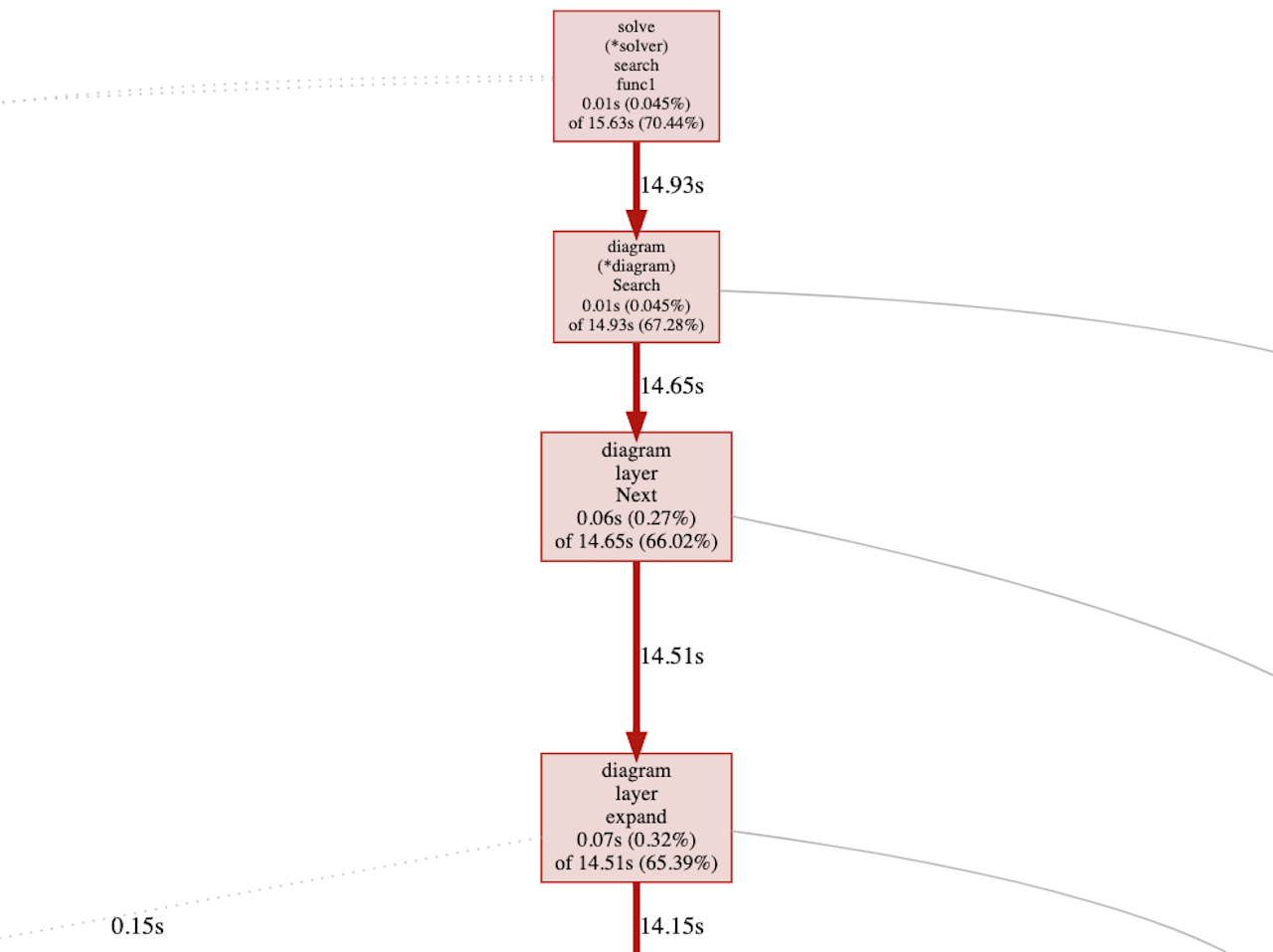
By looking at the graph, we can gain insight into how much time each function call is taking to execute. Note that the image above is but a small preview; the full graph is much larger.

For an alternate view, navigate to http://localhost:6060/ui/flamegraph:

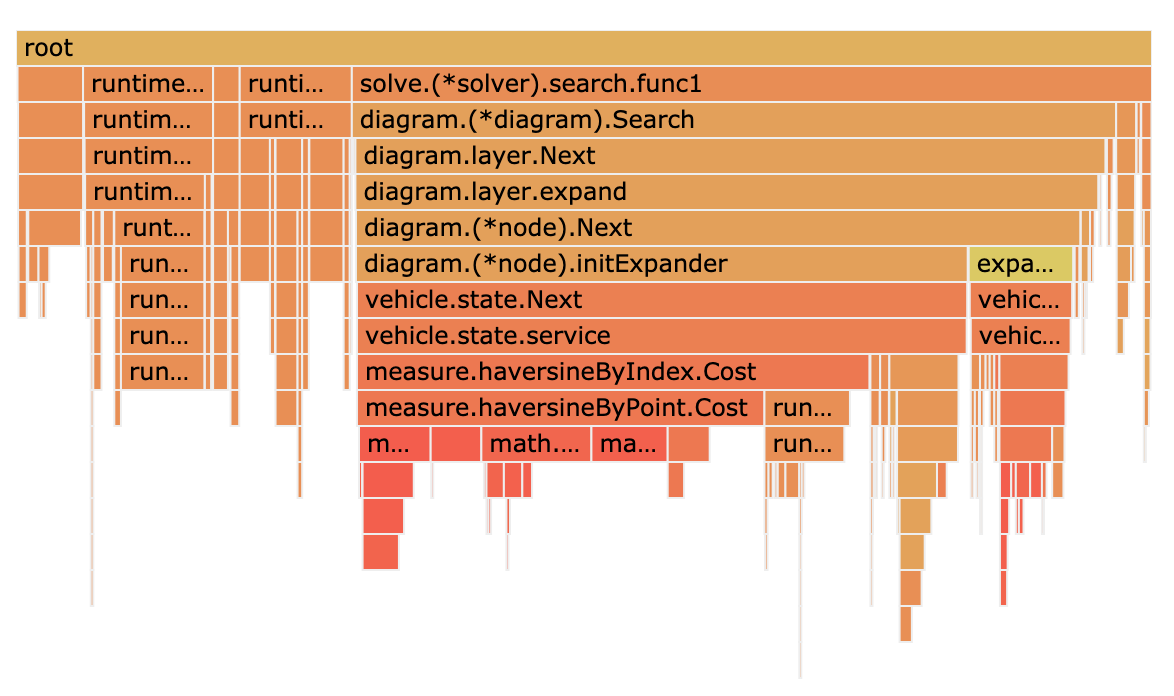
This type of graph is preferred by those who might find the previous chart a bit ungainly. Hovering a mouse cursor over a node displays the accumulated time the function took to execute while samples were being collected.

Let's look at another example from Dash.

Navigate to the code/dash/examples/queue directory. First, like before, we need to create our profile data file:

cat input.json | ./queue -dash.simulator.limits.duration 1s \
                         -dash.runner.profile.cpu queue.prof

Now, let's run pprof so we can see how our simulation may be tweaked. queue in the example below refers to the binary created when running go build in code/dash/examples/queue, while queue.prof is the profile data file created by adding -dash-runner.profile.cpu queue.prof when executing a Dash simulation.

go tool pprof -http localhost:6060 queue queue.prof

When the page loads, let's navigate to the flame graph http://localhost:6060/ui/flamegraph:

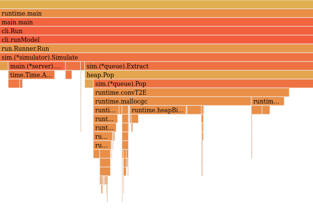
As above, hovering a mouse cursor over a node displays the accumulated time the function took to execute while samples were being collected.

This section should suffice as an introduction to this powerful tool. For more in-depth documentation, visit Go's official pprof package page, or the Go Blog entry "Profiling Go Programs".